End-to-End Regression
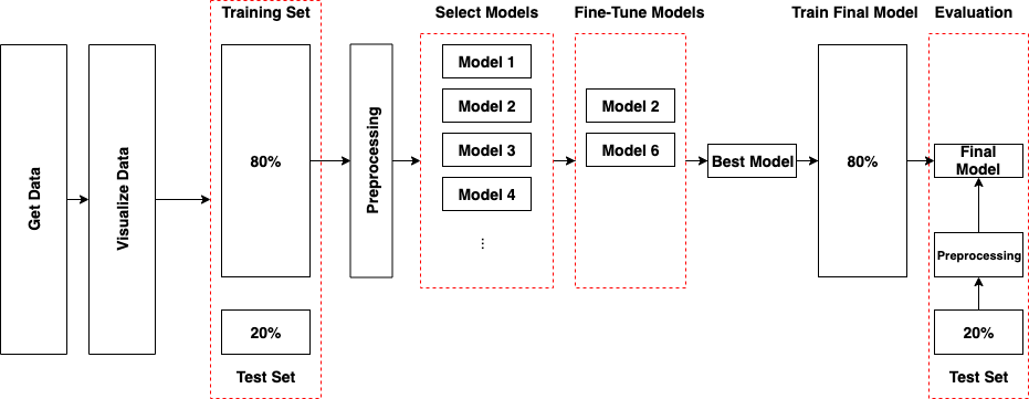
1. Get the Data

In [145]:
import pandas as pd

data = pd.read_csv('housing.csv') # California Housing Prices
data.head()
Out[145]:
longitude latitude housing_median_age total_rooms total_bedrooms population households median_income median_house_value ocean_proximity
0 -122.23 37.88 41.0 880.0 129.0 322.0 126.0 8.3252 452600.0 NEAR BAY
1 -122.22 37.86 21.0 7099.0 1106.0 2401.0 1138.0 8.3014 358500.0 NEAR BAY
2 -122.24 37.85 52.0 1467.0 190.0 496.0 177.0 7.2574 352100.0 NEAR BAY
3 -122.25 37.85 52.0 1274.0 235.0 558.0 219.0 5.6431 341300.0 NEAR BAY
4 -122.25 37.85 52.0 1627.0 280.0 565.0 259.0 3.8462 342200.0 NEAR BAY
In [19]:
data.info()
# total_bedrooms has only 20,433 non-null values meaning that 207 districts, need to take care of this
# ocean_proximity is a categorical attribute
<class 'pandas.core.frame.DataFrame'>
RangeIndex: 20640 entries, 0 to 20639
Data columns (total 10 columns):
longitude             20640 non-null float64
latitude              20640 non-null float64
housing_median_age    20640 non-null float64
total_rooms           20640 non-null float64
total_bedrooms        20433 non-null float64
population            20640 non-null float64
households            20640 non-null float64
median_income         20640 non-null float64
median_house_value    20640 non-null float64
ocean_proximity       20640 non-null object
dtypes: float64(9), object(1)
memory usage: 1.6+ MB
In [20]:
# check categorical attribute
data["ocean_proximity"].value_counts()
Out[20]:
<1H OCEAN     9136
INLAND        6551
NEAR OCEAN    2658
NEAR BAY      2290
ISLAND           5
Name: ocean_proximity, dtype: int64
In [21]:
# show a summary of the numerical attributes
data.describe()
Out[21]:
longitude latitude housing_median_age total_rooms total_bedrooms population households median_income median_house_value
count 20640.000000 20640.000000 20640.000000 20640.000000 20433.000000 20640.000000 20640.000000 20640.000000 20640.000000
mean -119.569704 35.631861 28.639486 2635.763081 537.870553 1425.476744 499.539680 3.870671 206855.816909
std 2.003532 2.135952 12.585558 2181.615252 421.385070 1132.462122 382.329753 1.899822 115395.615874
min -124.350000 32.540000 1.000000 2.000000 1.000000 3.000000 1.000000 0.499900 14999.000000
25% -121.800000 33.930000 18.000000 1447.750000 296.000000 787.000000 280.000000 2.563400 119600.000000
50% -118.490000 34.260000 29.000000 2127.000000 435.000000 1166.000000 409.000000 3.534800 179700.000000
75% -118.010000 37.710000 37.000000 3148.000000 647.000000 1725.000000 605.000000 4.743250 264725.000000
max -114.310000 41.950000 52.000000 39320.000000 6445.000000 35682.000000 6082.000000 15.000100 500001.000000
In [22]:
plots = data.hist(bins = 50, figsize = (20, 15))

2. Discover and visualize the data to gain insights

In [23]:
import matplotlib.pyplot as plt
x = data['longitude']
y = data['latitude']
data.plot(kind='scatter', x='longitude', y='latitude', alpha=0.4, label='population', figsize=(10, 7), c='median_house_value', cmap=plt.get_cmap('jet'), colorbar=True)
Out[23]:
<matplotlib.axes._subplots.AxesSubplot at 0x1a250502d0>
In [24]:
# Add more Attributie Combinations which have higher Correlation with median_house_value
data_copy = data.copy()
data_copy["rooms_per_household"] = data_copy["total_rooms"]/data_copy["households"]
data_copy["bedrooms_per_room"] = data_copy["total_bedrooms"]/data_copy["total_rooms"]
data_copy["population_per_household"]=data_copy["population"]/data_copy["households"]
In [25]:
# Looking for Correlations or Use scatter_matrix
corr_matrix = data_copy.corr()
corr_matrix['median_house_value']
Out[25]:
longitude                  -0.045967
latitude                   -0.144160
housing_median_age          0.105623
total_rooms                 0.134153
total_bedrooms              0.049686
population                 -0.024650
households                  0.065843
median_income               0.688075
median_house_value          1.000000
rooms_per_household         0.151948
bedrooms_per_room          -0.255880
population_per_household   -0.023737
Name: median_house_value, dtype: float64
In [35]:
# Looking for Correlations or Use scatter_matrix
corr_matrix = data_copy.corr()

import seaborn as sns
fig, ax = plt.subplots(figsize=(10,10))
sns.heatmap(corr_matrix, vmax=0.1, center=0, fmt='.2f',
                square=False, linewidths=.5, annot=True, cbar_kws={"shrink": 0.7}, ax = ax)
Out[35]:
<matplotlib.axes._subplots.AxesSubplot at 0x1a27d09950>

Feature Selection

  • the process of selecting the attributes that can make the predicted variable more accurate or eliminating those attributes that are irrelevant and can decrease the model accuracy and quality

Data Correlation

  • Correlation can help in predicting one attribute from another
  • Correlation can (sometimes) indicate the presence of a causal relationship
  • Correlation is used as a basic quantity for many modelling techniques
  • If your dataset has perfectly positive or negative attributes, the performance of the model will be impacted by multicollinearity. Luckily, decision trees and boosted trees algorithms are immune to multicollinearity by nature.
    • The easiest way is to delete or eliminate one of the perfectly correlated features
    • use a dimension reduction algorithm such as Principle Component Analysis (PCA)

Correlation

  • Pearson Correlation Coefficient, used with continuous variables that have a linear relationship
  • Spearman Correlation Coefficient, used with variable that have a non-linear relationship

3. Prepare Training Set and Test Set

In [280]:
# Read Data
data = pd.read_csv('housing.csv')

# Create Training Set and Test Set

from sklearn.model_selection import train_test_split
# train_test_split
# test_size, ratio of test set
# train_size, ratio of trainning set
# random_state, random seed
# shuffle, whether or not to shuffle the data before splitting
# stratify, data is split in a stratified fashion

import numpy as np
data_X = data.drop(['median_house_value'], axis = 1) # DataFrame
data_Y = data['median_house_value'] # Series

# split the dataset by categories of median income
data['income_cat'] = np.ceil(data['median_income']/1.5)
data['income_cat'].where(data['income_cat'] < 5, 5, inplace=True)

train_X, test_X, train_Y, test_Y = train_test_split(data_X, data_Y, test_size=0.2, random_state=42, stratify = data['income_cat'])

4. Prepare the Data for Machine Learning Algorithms

In [281]:
#Custom Transformer, add three features

from sklearn.base import BaseEstimator, TransformerMixin

class AddAttributes(BaseEstimator, TransformerMixin):
    def __init__(self): # no *args or **kargs
        pass
    def fit(self, X, y=None):
        return self  # nothing else to do
    def transform(self, X):
        X["rooms_per_household"] = X["total_rooms"]/X["households"]
        X["bedrooms_per_room"] = X["total_bedrooms"]/X["total_rooms"]
        X["population_per_household"]=X["population"]/X["households"]
        return X
In [140]:
train_X_num = train_X.drop("ocean_proximity", axis=1)
attr_adder = AddAttributes()
temp = attr_adder.transform(data_num)
In [141]:
# Data Cleaning
from sklearn.impute import SimpleImputer

imputer = SimpleImputer(strategy="median")
temp_2 = imputer.fit_transform(train_X_num)
In [142]:
# Convert Text and Categorical Attributes to Dummy Attributes
from sklearn.preprocessing import LabelBinarizer

encoder = LabelBinarizer()
temp_3 = encoder.fit_transform(train_X['ocean_proximity'])

Scaling variables

  • zero-mean normalization: $x_{i}=(x_{i}−mean(x_{i}))/std(x_{i})$, standardization
  • Min-max normalization: $x_{i}=(x_{i}−min(x_{i})/(max(x_{i})−min(x_{i}))$ normalizaiton, recommendation
In [143]:
# feature scaling
from sklearn.preprocessing import MinMaxScaler

scaler = MinMaxScaler()
temp_4 = scaler.fit_transform(train_X_num)

Transformation Pipelines

In [282]:
class DataFrameSelector(BaseEstimator, TransformerMixin):
    def __init__(self, attribute_names):
        self.attribute_names = attribute_names
    def fit(self, X, y=None):
        return self
    def transform(self, X):
        return X[self.attribute_names]
In [283]:
# Create Pipeline for Numeric Columns
from sklearn.pipeline import Pipeline
from sklearn.impute import SimpleImputer
from sklearn.preprocessing import StandardScaler

num_pipeline = Pipeline([
    ("select_numeric", DataFrameSelector(['longitude','latitude','housing_median_age','total_rooms','total_bedrooms','population','households','median_income',])),
    ('attribs_adder', AddAttributes()),
    ('imputer', SimpleImputer(strategy="median")),
    ('std_scaler', StandardScaler()),
])

#train_X_tr = num_pipeline.fit_transform(train_X)
In [284]:
# Create Pipeline for Categorical Columns
from sklearn.preprocessing import OneHotEncoder

cat_pipeline = Pipeline([
    ("select_numeric", DataFrameSelector(['ocean_proximity'])),
    ('cat', OneHotEncoder()),
])

#data_cat_tr = cat_pipeline.fit_transform(train_X)
In [285]:
# Merge Numeric Columns and Categorical Columns
from sklearn.pipeline import FeatureUnion

preprocess_pipeline = FeatureUnion(transformer_list=[
        ("num_pipeline", num_pipeline),
        ("cat_pipeline", cat_pipeline),
    ])
In [286]:
train_X = preprocess_pipeline.fit_transform(train_X).toarray()

5. Select and Train a Model

  • Do not spending too much time tweaking the hyperparameters, the goal is to shortlist a few promissing models
In [287]:
models = [] # save models

from sklearn.linear_model import LinearRegression
models.append(LinearRegression()) # linear regression model

from sklearn.tree import DecisionTreeRegressor
models.append(DecisionTreeRegressor(random_state=42)) # decision tree model

from sklearn.ensemble import RandomForestRegressor # random forest model
models.append(RandomForestRegressor())

from sklearn.svm import SVR
models.append(SVR(kernel="linear")) # Support Vector Regression model
In [225]:
from sklearn.model_selection import cross_val_score

def cross_validation(model, X, Y, k = 10):
    scores = cross_val_score(model, X, Y, scoring='neg_mean_squared_error', cv = k);
    return np.sqrt(-scores).mean(), np.sqrt(-scores).std() # represent perforance and precision respectively
In [228]:
for model in models:
    mean, std = cross_validation(model, train_X, train_Y, 10)
    print(mean, std)
68480.58471553595 2845.5843092650834
71035.2888883461 2456.17961798448
/opt/anaconda3/lib/python3.7/site-packages/sklearn/ensemble/forest.py:245: FutureWarning: The default value of n_estimators will change from 10 in version 0.20 to 100 in 0.22.
  "10 in version 0.20 to 100 in 0.22.", FutureWarning)
/opt/anaconda3/lib/python3.7/site-packages/sklearn/ensemble/forest.py:245: FutureWarning: The default value of n_estimators will change from 10 in version 0.20 to 100 in 0.22.
  "10 in version 0.20 to 100 in 0.22.", FutureWarning)
/opt/anaconda3/lib/python3.7/site-packages/sklearn/ensemble/forest.py:245: FutureWarning: The default value of n_estimators will change from 10 in version 0.20 to 100 in 0.22.
  "10 in version 0.20 to 100 in 0.22.", FutureWarning)
/opt/anaconda3/lib/python3.7/site-packages/sklearn/ensemble/forest.py:245: FutureWarning: The default value of n_estimators will change from 10 in version 0.20 to 100 in 0.22.
  "10 in version 0.20 to 100 in 0.22.", FutureWarning)
/opt/anaconda3/lib/python3.7/site-packages/sklearn/ensemble/forest.py:245: FutureWarning: The default value of n_estimators will change from 10 in version 0.20 to 100 in 0.22.
  "10 in version 0.20 to 100 in 0.22.", FutureWarning)
/opt/anaconda3/lib/python3.7/site-packages/sklearn/ensemble/forest.py:245: FutureWarning: The default value of n_estimators will change from 10 in version 0.20 to 100 in 0.22.
  "10 in version 0.20 to 100 in 0.22.", FutureWarning)
/opt/anaconda3/lib/python3.7/site-packages/sklearn/ensemble/forest.py:245: FutureWarning: The default value of n_estimators will change from 10 in version 0.20 to 100 in 0.22.
  "10 in version 0.20 to 100 in 0.22.", FutureWarning)
/opt/anaconda3/lib/python3.7/site-packages/sklearn/ensemble/forest.py:245: FutureWarning: The default value of n_estimators will change from 10 in version 0.20 to 100 in 0.22.
  "10 in version 0.20 to 100 in 0.22.", FutureWarning)
/opt/anaconda3/lib/python3.7/site-packages/sklearn/ensemble/forest.py:245: FutureWarning: The default value of n_estimators will change from 10 in version 0.20 to 100 in 0.22.
  "10 in version 0.20 to 100 in 0.22.", FutureWarning)
/opt/anaconda3/lib/python3.7/site-packages/sklearn/ensemble/forest.py:245: FutureWarning: The default value of n_estimators will change from 10 in version 0.20 to 100 in 0.22.
  "10 in version 0.20 to 100 in 0.22.", FutureWarning)
52547.86132487167 1771.793006493265
111711.14888265522 2754.3053045240267

6. Fine-Tune Your Model

  • Select a couple of models having reasonable performance from above
  • Fine-tune these models to generate the best model
In [260]:
from sklearn.model_selection import GridSearchCV

param_grid = [{'n_estimators': [40, 50, 100], 'max_features': [2, 4, 6, 8, 10, 12]}]

grid_search = GridSearchCV(RandomForestRegressor(), param_grid, cv=5, scoring='neg_mean_squared_error')

grid_search.fit(train_X, train_Y)
Out[260]:
GridSearchCV(cv=5, error_score='raise-deprecating',
             estimator=RandomForestRegressor(bootstrap=True, criterion='mse',
                                             max_depth=None,
                                             max_features='auto',
                                             max_leaf_nodes=None,
                                             min_impurity_decrease=0.0,
                                             min_impurity_split=None,
                                             min_samples_leaf=1,
                                             min_samples_split=2,
                                             min_weight_fraction_leaf=0.0,
                                             n_estimators='warn', n_jobs=None,
                                             oob_score=False, random_state=None,
                                             verbose=0, warm_start=False),
             iid='warn', n_jobs=None,
             param_grid=[{'max_features': [2, 4, 6, 8, 10, 12],
                          'n_estimators': [40, 50, 100]},
                         {'bootstrap': [False], 'max_features': [2, 3, 4],
                          'n_estimators': [3, 10]}],
             pre_dispatch='2*n_jobs', refit=True, return_train_score=False,
             scoring='neg_mean_squared_error', verbose=0)
In [261]:
grid_search.best_params_ # best combination of parameters
Out[261]:
{'max_features': 8, 'n_estimators': 100}
In [262]:
grid_search.best_estimator_ # best model
# If GridSearchCV is initialized with refit=Ture (which is the default), 
# then once it finds the best estimator using cross-validation, it retrains it on the whole training set
Out[262]:
RandomForestRegressor(bootstrap=True, criterion='mse', max_depth=None,
                      max_features=8, max_leaf_nodes=None,
                      min_impurity_decrease=0.0, min_impurity_split=None,
                      min_samples_leaf=1, min_samples_split=2,
                      min_weight_fraction_leaf=0.0, n_estimators=100,
                      n_jobs=None, oob_score=False, random_state=None,
                      verbose=0, warm_start=False)
In [274]:
# evaluation scores
cvres = grid_search.cv_results_
for mean_score, params in zip(cvres["mean_test_score"], cvres["params"]):
    print(np.sqrt(-mean_score), params)
52527.28987688461 {'max_features': 2, 'n_estimators': 40}
52169.78960548942 {'max_features': 2, 'n_estimators': 50}
51869.6403052311 {'max_features': 2, 'n_estimators': 100}
50273.34680132435 {'max_features': 4, 'n_estimators': 40}
50037.19119510559 {'max_features': 4, 'n_estimators': 50}
49706.25065507569 {'max_features': 4, 'n_estimators': 100}
49538.25159971055 {'max_features': 6, 'n_estimators': 40}
49504.248668628956 {'max_features': 6, 'n_estimators': 50}
49420.464219225876 {'max_features': 6, 'n_estimators': 100}
49654.645579303025 {'max_features': 8, 'n_estimators': 40}
49749.622469891874 {'max_features': 8, 'n_estimators': 50}
49087.967725059374 {'max_features': 8, 'n_estimators': 100}
49760.16249539341 {'max_features': 10, 'n_estimators': 40}
49908.43115880318 {'max_features': 10, 'n_estimators': 50}
49420.56682885718 {'max_features': 10, 'n_estimators': 100}
50235.659286418755 {'max_features': 12, 'n_estimators': 40}
49846.19047685978 {'max_features': 12, 'n_estimators': 50}
49756.23251404187 {'max_features': 12, 'n_estimators': 100}
62016.77154099544 {'bootstrap': False, 'max_features': 2, 'n_estimators': 3}
53762.06411973067 {'bootstrap': False, 'max_features': 2, 'n_estimators': 10}
59351.5858886507 {'bootstrap': False, 'max_features': 3, 'n_estimators': 3}
52812.88158905331 {'bootstrap': False, 'max_features': 3, 'n_estimators': 10}
58758.336757269724 {'bootstrap': False, 'max_features': 4, 'n_estimators': 3}
51521.058259005986 {'bootstrap': False, 'max_features': 4, 'n_estimators': 10}
In [237]:
# Select a random combination of hyperparameter at every iteration
from sklearn.model_selection import RandomizedSearchCV

param_random = {'n_estimators': [50, 100, 150], 'max_features': [2, 4, 6, 8, 10, 12]}

random_search = RandomizedSearchCV(RandomForestRegressor(), param_random, cv=5, scoring='neg_mean_squared_error', n_iter = 10)

random_search.fit(train_X, train_Y)
Out[237]:
RandomizedSearchCV(cv=5, error_score='raise-deprecating',
                   estimator=RandomForestRegressor(bootstrap=True,
                                                   criterion='mse',
                                                   max_depth=None,
                                                   max_features='auto',
                                                   max_leaf_nodes=None,
                                                   min_impurity_decrease=0.0,
                                                   min_impurity_split=None,
                                                   min_samples_leaf=1,
                                                   min_samples_split=2,
                                                   min_weight_fraction_leaf=0.0,
                                                   n_estimators='warn',
                                                   n_jobs=None, oob_score=False,
                                                   random_state=None, verbose=0,
                                                   warm_start=False),
                   iid='warn', n_iter=10, n_jobs=None,
                   param_distributions={'max_features': [2, 4, 6, 8, 10, 12],
                                        'n_estimators': [50, 100, 150]},
                   pre_dispatch='2*n_jobs', random_state=None, refit=True,
                   return_train_score=False, scoring='neg_mean_squared_error',
                   verbose=0)
In [238]:
random_search.best_params_ # best combination of parameters
Out[238]:
{'n_estimators': 150, 'max_features': 6}
In [239]:
cvres = random_search.cv_results_
for mean_score, params in zip(cvres["mean_test_score"], cvres["params"]):
    print(np.sqrt(-mean_score), params)
51728.70993263402 {'n_estimators': 100, 'max_features': 2}
49499.19408833201 {'n_estimators': 50, 'max_features': 8}
49636.25379861854 {'n_estimators': 50, 'max_features': 6}
49410.96742527571 {'n_estimators': 150, 'max_features': 10}
49115.81496692589 {'n_estimators': 150, 'max_features': 6}
49582.48906382619 {'n_estimators': 100, 'max_features': 10}
49781.290845521806 {'n_estimators': 100, 'max_features': 12}
52282.97103341898 {'n_estimators': 50, 'max_features': 2}
49761.92632748126 {'n_estimators': 150, 'max_features': 12}
50217.99942408262 {'n_estimators': 50, 'max_features': 4}

7. Ensemble Methods

8. Analyze the Best Models and Their Errors

In [74]:
# Look at the specific errors, try to understand why it makes them and what could fix the problem, 
# e.g., adding extra features or getting rid of uninformative ones, cleaning up outliers
feature_importance = grid_search.best_estimator_.feature_importances_
l = zip(feature_importance, data_X.columns)
for e in l:
    print(e)
(0.06987224280924181, 'longitude')
(0.061471397171406934, 'latitude')
(0.04468273895530531, 'housing_median_age')
(0.014873871910961602, 'total_rooms')
(0.014229130715786674, 'total_bedrooms')
(0.014463135495184269, 'population')
(0.014194876364158223, 'households')
(0.36755846701801076, 'median_income')
(0.04875775134279811, 'ocean_proximity')
(0.06202679118353847, 'income_cat')

9. Train Final Model

In [288]:
final_model = grid_search.best_estimator_
#final_model.fit(train_X, train_Y) # Do not have to retain, it has been done by GridSearchCV or RandomizedSearchCV

10. Evaluate System on the Test Set

In [289]:
test_X = preprocess_pipeline.transform(test_X).toarray()
In [290]:
# Evaluate test dataset
from sklearn.metrics import mean_squared_error

predictions = final_model.predict(test_X)

MSE = mean_squared_error(test_Y, predictions)
RMSE = np.sqrt(MSE)
RMSE
Out[290]:
47081.741234699286
In [291]:
# 95% confidence interval for the generalizaiton error
from scipy import stats

confidence = 0.95
squared_errors = (predictions - test_Y) ** 2
np.sqrt(stats.t.interval(confidence, len(squared_errors) - 1,
                         loc=squared_errors.mean(),
                         scale=stats.sem(squared_errors)))
Out[291]:
array([45096.96449215, 48986.16650623])

11. Deliver Model

In [271]:
import pickle
 
f = open('model.pkl', 'wb');
pickle.dump(final_model, f, -1);
In [ ]:
import joblib

jolib.dump(final_model, 'model.pkl')

#model_loaded = joblib.load('model.pkl')