SVM

Converted to

$$min(\dfrac{1}{2}w^{T}w + C\Sigma_{i=1}^{m}\zeta^{i})$$

• w is the weight vector
• $\zeta$ is the slack variables, control the margin violation

Subject to $$t^{(i)}(w^{T}x^{(i)} + b) \geq 1 - \zeta^{i}$$

Linear SVM Classification

• No Kernel

from sklearn.svm import SVC # kernel = 'linear'
from sklearn.svm import LinearSVC
from sklearn.linear_model import SGDClassifier # loss = 'hinge', alpha=1/(m*C)

from sklearn.svm import SVC
from sklearn import datasets

iris = datasets.load_iris()
X = iris["data"][:, (2, 3)]  # petal length, petal width
y = iris["target"]

setosa_or_versicolor = (y == 0) | (y == 1)
X = X[setosa_or_versicolor]
y = y[setosa_or_versicolor]

# SVM Classifier model
svm_clf = SVC(kernel="linear", C=float("inf")) # no regulation
svm_clf.fit(X, y)

SVC(C=inf, cache_size=200, class_weight=None, coef0=0.0,
    decision_function_shape='ovr', degree=3, gamma='auto_deprecated',
    kernel='linear', max_iter=-1, probability=False, random_state=None,
    shrinking=True, tol=0.001, verbose=False)

import matplotlib.pyplot as plt
import numpy as np

def plot_svc_decision_boundary(X, y, svm_clf, xmin, xmax):
    w = svm_clf.coef_[0]
    b = svm_clf.intercept_[0]

    # At the decision boundary, w0*x0 + w1*x1 + b = 0
    # => x1 = -w0/w1 * x0 - b/w1
    x0 = np.linspace(xmin, xmax, 200)
    decision_boundary = -w[0]/w[1] * x0 - b/w[1]

    margin = 1/w[1]
    gutter_up = decision_boundary + margin
    gutter_down = decision_boundary - margin

    svs = svm_clf.support_vectors_
    plt.scatter(svs[:, 0], svs[:, 1], s=180, facecolors='#FFAAAA')
    plt.plot(x0, decision_boundary, "k-", linewidth=2)
    plt.plot(x0, gutter_up, "k--", linewidth=2)
    plt.plot(x0, gutter_down, "k--", linewidth=2)
    plt.plot(X[:, 0][y==1], X[:, 1][y==1], "bs")
    plt.plot(X[:, 0][y==0], X[:, 1][y==0], "yo")
    
plot_svc_decision_boundary(X, y, svm_clf, 0, 5.5)
plt.axis([0, 5.5, 0, 2])

[0, 5.5, 0, 2]

Soft Margin Classification

• Find a good balance between keeping the street as large as possible and limiting the margin violations (i.e., instances that end up in the middle of the street or even on the wrong side)
• Scikit-Learn SVM control the balance using the C parameter
  • small C, wider street, more margin violations
  • large C, smaller street, fewer margin violations
  • overfitting, reduce C
• SVMs are sensitive to the feature scales

from sklearn.preprocessing import StandardScaler
scaler = StandardScaler()
X_scale = scaler.fit_transform(X)

from sklearn.svm import LinearSVC

# LinearSVC uses liblinear rather than libsvm, more flexibility, faster than SVC(kernel='linear')
# Or use SGDClassifier(loss='hinge', alpha=1/(m*C))
svm_clf1 = LinearSVC(C=1, loss="hinge", random_state=42)
svm_clf1.fit(X, y)
svm_clf2 = LinearSVC(C=100, loss="hinge", random_state=42)
svm_clf2.fit(X, y)

LinearSVC(C=100, class_weight=None, dual=True, fit_intercept=True,
          intercept_scaling=1, loss='hinge', max_iter=1000, multi_class='ovr',
          penalty='l2', random_state=42, tol=0.0001, verbose=0)

def plot_svc_decision_boundary(X, y, svm_clf, xmin, xmax):
    w = svm_clf.coef_[0]
    b = svm_clf.intercept_[0]

    # At the decision boundary, w0*x0 + w1*x1 + b = 0
    # => x1 = -w0/w1 * x0 - b/w1
    x0 = np.linspace(xmin, xmax, 200)
    decision_boundary = -w[0]/w[1] * x0 - b/w[1]

    margin = 1/w[1]
    gutter_up = decision_boundary + margin
    gutter_down = decision_boundary - margin

    #svs = svm_clf.support_vectors_
    #plt.scatter(svs[:, 0], svs[:, 1], s=180, facecolors='#FFAAAA')
    plt.plot(x0, decision_boundary, "k-", linewidth=2)
    plt.plot(x0, gutter_up, "k--", linewidth=2)
    plt.plot(x0, gutter_down, "k--", linewidth=2)
    plt.plot(X[:, 0][y==1], X[:, 1][y==1], "bs")
    plt.plot(X[:, 0][y==0], X[:, 1][y==0], "yo")

plot_svc_decision_boundary(X, y, svm_clf1, 0, 5.5) # C = 1

plot_svc_decision_boundary(X, y, svm_clf2, 0, 5.5) # C = 100

Polynomial Kernel Function

from sklearn.datasets import make_moons
X, y = make_moons(n_samples=100, noise=0.15, random_state=42)

def plot_dataset(X, y, axes):
    plt.plot(X[:, 0][y==0], X[:, 1][y==0], "bs")
    plt.plot(X[:, 0][y==1], X[:, 1][y==1], "g^")
    plt.axis(axes)
    plt.grid(True, which='both')
    plt.xlabel(r"$x_1$", fontsize=20)
    plt.ylabel(r"$x_2$", fontsize=20, rotation=0)
    
plot_dataset(X, y, [-1.5, 2.5, -1, 1.5])

from sklearn.datasets import make_moons
from sklearn.pipeline import Pipeline
from sklearn.preprocessing import PolynomialFeatures

polynomial_svm_clf = Pipeline([
        ("poly_features", PolynomialFeatures(degree=3)),
        ("scaler", StandardScaler()),
        ("svm_clf", LinearSVC(C=10, loss="hinge", random_state=42))
    ])

polynomial_svm_clf.fit(X, y)

Pipeline(memory=None,
         steps=[('poly_features',
                 PolynomialFeatures(degree=3, include_bias=True,
                                    interaction_only=False, order='C')),
                ('scaler',
                 StandardScaler(copy=True, with_mean=True, with_std=True)),
                ('svm_clf',
                 LinearSVC(C=10, class_weight=None, dual=True,
                           fit_intercept=True, intercept_scaling=1,
                           loss='hinge', max_iter=1000, multi_class='ovr',
                           penalty='l2', random_state=42, tol=0.0001,
                           verbose=0))],
         verbose=False)

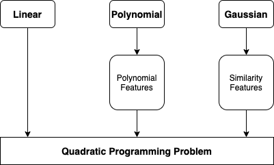
• Polynomial features work great with all sort of Machine Learning algorithms
• Creating a huge number features makes the model too slow
• SVC with kernel='poly', same as adding polynomial features without actually adding them

from sklearn.pipeline import Pipeline

poly_kernel_svm_clf = Pipeline([
        ("scaler", StandardScaler()),
        ("svm_clf", SVC(kernel="poly", degree=3, coef0=1, C=5)) 
        # coef0 controls how much the model is influenced by high-degree polynomials versus low-degree polynomials
    ])

poly_kernel_svm_clf.fit(X, y)

Pipeline(memory=None,
         steps=[('scaler',
                 StandardScaler(copy=True, with_mean=True, with_std=True)),
                ('svm_clf',
                 SVC(C=5, cache_size=200, class_weight=None, coef0=1,
                     decision_function_shape='ovr', degree=3,
                     gamma='auto_deprecated', kernel='poly', max_iter=-1,
                     probability=False, random_state=None, shrinking=True,
                     tol=0.001, verbose=False))],
         verbose=False)

def plot_predictions(clf, axes):
    x0s = np.linspace(axes[0], axes[1], 100)
    x1s = np.linspace(axes[2], axes[3], 100)
    x0, x1 = np.meshgrid(x0s, x1s)
    X = np.c_[x0.ravel(), x1.ravel()]
    y_pred = clf.predict(X).reshape(x0.shape)
    y_decision = clf.decision_function(X).reshape(x0.shape)
    plt.contourf(x0, x1, y_pred, cmap=plt.cm.brg, alpha=0.2)
    plt.contourf(x0, x1, y_decision, cmap=plt.cm.brg, alpha=0.1)
    
plot_predictions(poly_kernel_svm_clf, [-1.5, 2.5, -1, 1.5])
plot_dataset(X, y, [-1.5, 2.5, -1, 1.5])

Gaussian Radial Basis Kernel Function (RBF)

• SVC use kernel trick to obtain a similar result as if adding many similarity features
• gamma, kernel coefficient for ‘rbf’, ‘poly’ and ‘sigmoid’
  • rbf, gamma = 1/lamda, small gamma, large lamda, high bias, low variance
  • increasing gamma makes the bell-shaped curve narrower, the influence of each instance is smaller
  • overfitting, reduce gamma

Computational Complexity

• LinearSVC, O(mn)
• SGDClassifier, O(mn)
• SVC, $O(m^{2}*n)$ to $O(m^{3}*n)$

SVM Regression

• Fit as many instance as possible on the street while limiting margin violations (i.e., instances off the street)
• LinearSVR
• SVR

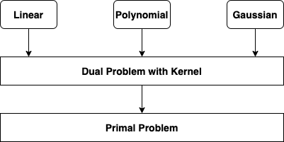
Kernel

• Kernel is a function capable of computing the dot product $\phi(a)^{T} \phi(b)$, based only on the original vectors a and b, without having to compute the transformation $\phi$
• Linear: $K(a, b) = a^{T}b$
• Polynomial: $K(a, b) = (\gamma a^{T}b+r)^{d}$
• Gaussian RBF: $K(a, b) = exp(-\gamma \lVert{a-b}\rVert^{2})$
• Sigmoid: $K(a, b) = tanh(\gamma a^{T}b + r)$

Online SVMs

• SGDClassifier

Hinge Loss

• max(0, 1-t)