import warnings
warnings.filterwarnings('ignore')
from sktime.datasets import load_longley
_, y = load_longley() # 16*5
y.head()
| GNPDEFL | GNP | UNEMP | ARMED | POP | |
|---|---|---|---|---|---|
| Period | |||||
| 1947 | 83.0 | 234289.0 | 2356.0 | 1590.0 | 107608.0 |
| 1948 | 88.5 | 259426.0 | 2325.0 | 1456.0 | 108632.0 |
| 1949 | 88.2 | 258054.0 | 3682.0 | 1616.0 | 109773.0 |
| 1950 | 89.5 | 284599.0 | 3351.0 | 1650.0 | 110929.0 |
| 1951 | 96.2 | 328975.0 | 2099.0 | 3099.0 | 112075.0 |
from sktime.forecasting.model_selection import temporal_train_test_split
y_train, y_test = temporal_train_test_split(y, test_size=4) # hold out last 4 years
from sklearn.ensemble import RandomForestRegressor
from sktime.forecasting.compose import make_reduction
from sktime.performance_metrics.forecasting import mean_absolute_percentage_error
import numpy as np
regressor = RandomForestRegressor(n_jobs = 1)
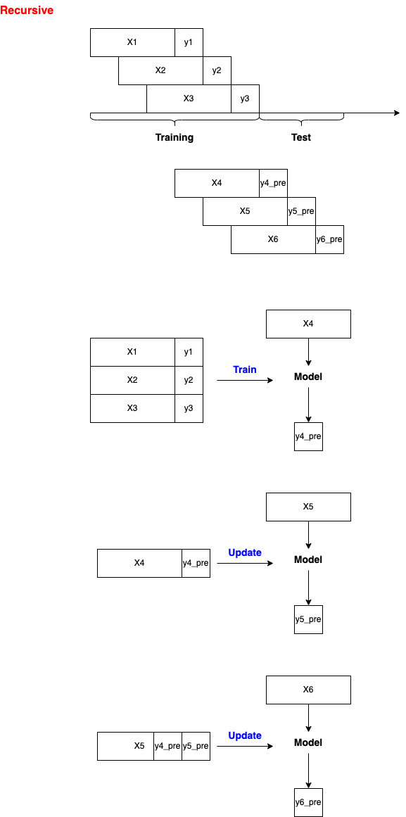
forecaster = make_reduction(regressor, window_length=6, strategy="recursive")
forecaster.fit(y_train)
RecursiveTabularRegressionForecaster(estimator=RandomForestRegressor(n_jobs=1),
                                     window_length=6)
In a Jupyter environment, please rerun this cell to show the HTML representation or trust the notebook. RecursiveTabularRegressionForecaster(estimator=RandomForestRegressor(n_jobs=1),
window_length=6)RandomForestRegressor(n_jobs=1)
RandomForestRegressor(n_jobs=1)
import numpy as np

fh = np.arange(1, 5)
y_pred = forecaster.predict(fh)
y_pred
| GNPDEFL | GNP | UNEMP | ARMED | POP | |
|---|---|---|---|---|---|
| Period | |||||
| 1959 | 2727.12 | 439302.0 | 109.71 | 121368.92 | 3702.11 |
| 1960 | 2737.10 | 439302.0 | 109.71 | 121368.92 | 3106.78 |
| 1961 | 2752.77 | 439302.0 | 109.71 | 121368.92 | 2925.72 |
| 1962 | 2752.77 | 439302.0 | 109.71 | 121368.92 | 2637.59 |
y_train.head()
| GNPDEFL | GNP | UNEMP | ARMED | POP | |
|---|---|---|---|---|---|
| Period | |||||
| 1947 | 83.0 | 234289.0 | 2356.0 | 1590.0 | 107608.0 |
| 1948 | 88.5 | 259426.0 | 2325.0 | 1456.0 | 108632.0 |
| 1949 | 88.2 | 258054.0 | 3682.0 | 1616.0 | 109773.0 |
| 1950 | 89.5 | 284599.0 | 3351.0 | 1650.0 | 110929.0 |
| 1951 | 96.2 | 328975.0 | 2099.0 | 3099.0 | 112075.0 |
# Re-order columns of prediction
y_pred = y_pred.iloc[:, [2, 1, 4, 0, 3]]
y_pred.columns = y_train.columns
y_pred
| GNPDEFL | GNP | UNEMP | ARMED | POP | |
|---|---|---|---|---|---|
| Period | |||||
| 1959 | 109.71 | 439302.0 | 3702.11 | 2727.12 | 121368.92 |
| 1960 | 109.71 | 439302.0 | 3106.78 | 2737.10 | 121368.92 |
| 1961 | 109.71 | 439302.0 | 2925.72 | 2752.77 | 121368.92 |
| 1962 | 109.71 | 439302.0 | 2637.59 | 2752.77 | 121368.92 |
from sktime.performance_metrics.forecasting import mean_absolute_percentage_error
mean_absolute_percentage_error(y_test, y_pred, symmetric=False, multioutput = 'raw_values')
array([0.04456511, 0.14409515, 0.24293608, 0.06347627, 0.04144224])
import matplotlib.pyplot as plt

def get_plots(y_train, y_test, y_pred):
    columns = list(y_train.columns)

    for column in columns:
        fig, ax = plt.subplots(figsize=(8, 6))
        line1, = ax.plot(y_train.index.to_timestamp(), y_train[column], 'bo-')
        line2, = ax.plot(y_test.index.to_timestamp(), y_test[column], 'go-')
        line3, = ax.plot(y_pred.index.to_timestamp(), y_pred[column], 'yo-')
        ax.legend((line1, line2, line3), ('y', 'y_test', 'y_pred'))
        ax.set_ylabel(column)

# visualization
get_plots(y_train, y_test, y_pred)


